Overview
This vignette walks through a compact, end-to-end grain-size analysis with grainsizeR. It uses the example files installed with the package and keeps each step as an ordinary R object so results can be checked, joined, plotted, and exported with standard R tools.
This vignette calls the primary public functions directly. Short aliases are available for interactive use, but the full function names are easier to read in scripts and reports. CRAN readiness is not claimed here.
Reading Long and Wide Grain-Size Data
Long input has one row per sample and size class. Wide input has one size column and one column per sample.
long_file <- system.file("extdata", "grain.long.csv", package = "grainsizeR")
wide_file <- system.file("extdata", "grain.wide.csv", package = "grainsizeR")

gs <- read_gsd(
  long_file,
  format = "long",
  sample_col = "sample",
  size_col = "size",
  value_col = "proportion",
  size_unit = "mm",
  value_type = "proportion"
)

gs_wide <- read_gsd_wide(
  wide_file,
  size_col = 1,
  size_unit = "mm",
  value_type = "percent"
)

head(gs)
#> # A tibble: 6 × 13
#>   sample_id bin_id raw_size_um size_lower_um size_upper_um size_mid_um
#>   <chr>      <int>       <dbl>         <dbl>         <dbl>       <dbl>
#> 1 S01            1        2000          2000            NA        NA
#> 2 S01            2        1000          1000          2000      1414.
#> 3 S01            3         500           500          1000       707.
#> 4 S01            4         250           250           500       354.
#> 5 S01            5         125           125           250       177.
#> 6 S01            6          63            63           125        88.7
#> # ℹ 7 more variables: size_mid_phi <dbl>, retained_percent <dbl>,
#> #   cum_finer_percent <dbl>, cum_coarser_percent <dbl>, is_open_lower <lgl>,
#> #   is_open_upper <lgl>, measurement_method <chr>
Inspecting and Validating gsd_tbl Objects
read_gsd() and read_gsd_wide() return
gsd_tbl objects. Diagnostics help identify open-ended
classes and threshold-resolution limits before running a large
analysis.
is_gsd_tbl(gs)
#> [1] TRUE
head(gs_diagnostics(gs, output = "summary"))
#> # A tibble: 6 × 8
#>   sample_id  n_ok n_warning n_error n_info has_error has_warning overall_status
#>   <chr>     <int>     <int>   <int>  <int> <lgl>     <lgl>       <chr>
#> 1 S01          24         5       0      2 FALSE     TRUE        warning
#> 2 S02          19         8       0      4 FALSE     TRUE        warning
#> 3 S03          19         8       0      4 FALSE     TRUE        warning
#> 4 S04          24         5       0      2 FALSE     TRUE        warning
#> 5 S05          24         5       0      2 FALSE     TRUE        warning
#> 6 S06          19         8       0      4 FALSE     TRUE        warning
Cumulative Percentages
gs_cumulative() returns finite-boundary cumulative
percentages by sample.
head(gs_cumulative(gs))
#> # A tibble: 6 × 7
#>   sample_id boundary_id boundary_um boundary_mm boundary_phi percent_finer
#>   <chr>           <int>       <dbl>       <dbl>        <dbl>         <dbl>
#> 1 S01                 1        2000       2            -1             99.4
#> 2 S01                 2        1000       1             0             98.4
#> 3 S01                 3         500       0.5           1             96.8
#> 4 S01                 4         250       0.25          2             77.7
#> 5 S01                 5         125       0.125         3             50.9
#> 6 S01                 6          63       0.063         3.99          14.4
#> # ℹ 1 more variable: percent_coarser <dbl>
D-Values and GRADISTAT-Style D-Spread Descriptors
Use gs_d_values() for requested percentiles and
gs_d_spread() for GRADISTAT-style D-ratio and D-difference
descriptors. Open-ended tails require an explicit extrapolation choice
when a requested value falls outside resolved boundaries.
head(suppressWarnings(gs_d_values(
  gs,
  probs = c(10, 50, 90),
  extrapolate = "warn_linear"
)))
#> # A tibble: 6 × 7
#>   sample_id percentile grain_size_um grain_size_mm grain_size_phi
#>   <chr>          <dbl>         <dbl>         <dbl>          <dbl>
#> 1 S01               10          40.9        0.0409           4.61
#> 2 S01               50         123.         0.123            3.02
#> 3 S01               90         390.         0.390            1.36
#> 4 S02               10          77.6        0.0776           3.69
#> 5 S02               50         175.         0.175            2.51
#> 6 S02               90         412.         0.412            1.28
#> # ℹ 2 more variables: interpolation_scale <chr>, extrapolated <lgl>

head(suppressWarnings(gs_d_spread(
  gs,
  extrapolate = "warn_linear"
)))
#> # A tibble: 6 × 15
#>   sample_id   D10   D25   D50   D75   D90 d_value_unit D90_D10_ratio
#>   <chr>     <dbl> <dbl> <dbl> <dbl> <dbl> <chr>                <dbl>
#> 1 S01        40.9  76.9  123.  233.  390. um                    9.54
#> 2 S02        77.6 114.   175.  267.  412. um                    5.30
#> 3 S03        69.5  91.3  151.  278.  402. um                    5.79
#> 4 S04        60.2  81.2  125.  258.  395. um                    6.56
#> 5 S05        62.2  80.1  123.  270.  410. um                    6.60
#> 6 S06        76.1 104.   216.  346.  439. um                    5.77
#> # ℹ 7 more variables: D90_minus_D10 <dbl>, D75_D25_ratio <dbl>,
#> #   D75_minus_D25 <dbl>, D90_D10_log_ratio <dbl>, D75_D25_log_ratio <dbl>,
#> #   quartile_deviation_phi <dbl>, any_extrapolated <lgl>
Folk and Ward Graphical Statistics
gs_folk_ward() calculates graphical statistics from
percentile estimates.
head(suppressWarnings(gs_folk_ward(
  gs,
  extrapolate = "warn_linear"
)))
#> # A tibble: 6 × 26
#>   sample_id D5_um D16_um D25_um D50_um D75_um D84_um D95_um D5_phi D16_phi
#>   <chr>     <dbl>  <dbl>  <dbl>  <dbl>  <dbl>  <dbl>  <dbl>  <dbl>   <dbl>
#> 1 S01        25.1   64.9   76.9   123.   233.   314.   468.   5.31    3.94
#> 2 S02        68.2   90.7  114.    175.   267.   346.   476.   3.87    3.46
#> 3 S03        63.5   77.5   91.3   151.   278.   347.   455.   3.98    3.69
#> 4 S04        32.3   69.6   81.2   125.   258.   333.   456.   4.95    3.85
#> 5 S05        35.3   68.7   80.1   123.   270.   347.   472.   4.82    3.86
#> 6 S06        68.5   86.2  104.    216.   346.   399.   475.   3.87    3.54
#> # ℹ 16 more variables: D25_phi <dbl>, D50_phi <dbl>, D75_phi <dbl>,
#> #   D84_phi <dbl>, D95_phi <dbl>, mean_fw_phi <dbl>, mean_fw_um <dbl>,
#> #   sorting_fw_phi <dbl>, skewness_fw <dbl>, kurtosis_fw <dbl>,
#> #   interpolation_scale <chr>, any_extrapolated <lgl>, mean_size_class <chr>,
#> #   sorting_class <chr>, skewness_class <chr>, kurtosis_class <chr>
Moment Statistics
Moment statistics require explicit open-end handling. This example extends terminal classes by one phi unit.
head(suppressWarnings(gs_moments(
  gs,
  open_end = "extend_phi"
)))
#> # A tibble: 6 × 14
#>   sample_id moment_method   mean_moment mean_moment_unit mean_moment_um
#>   <chr>     <chr>                 <dbl> <chr>                     <dbl>
#> 1 S01       logarithmic_phi        2.97 phi                        127.
#> 2 S02       logarithmic_phi        2.49 phi                        179.
#> 3 S03       logarithmic_phi        2.65 phi                        159.
#> 4 S04       logarithmic_phi        2.90 phi                        134.
#> 5 S05       logarithmic_phi        2.85 phi                        139.
#> 6 S06       logarithmic_phi        2.36 phi                        194.
#> # ℹ 9 more variables: mean_moment_phi <dbl>, sd_moment <dbl>,
#> #   sd_moment_unit <chr>, skewness_moment <dbl>, kurtosis_moment <dbl>,
#> #   retained_percent_used <dbl>, open_end <chr>, open_end_estimated <lgl>,
#> #   open_end_omitted <lgl>
Modes and Sample Modality
gs_modes() reports ranked retained-class modes and an
operational modality label.
head(gs_modes(gs))
#> # A tibble: 6 × 12
#>   sample_id sample_modality  mode_rank mode_size_mm mode_size_um mode_phi
#>   <chr>     <chr>                <int>        <dbl>        <dbl>    <dbl>
#> 1 S01       trimodal_or_more         1       0.0887         88.7     3.49
#> 2 S01       trimodal_or_more         2       0.177         177.      2.5
#> 3 S01       trimodal_or_more         3       0.354         354.      1.5
#> 4 S02       unimodal                 1       0.177         177.      2.5
#> 5 S02       unimodal                 2       0.0887         88.7     3.49
#> 6 S02       unimodal                 3       0.354         354.      1.5
#> # ℹ 6 more variables: mode_class_lower_mm <dbl>, mode_class_upper_mm <dbl>,
#> #   mode_percent <dbl>, mode_class_label <chr>, is_open_interval <lgl>,
#> #   mode_status <chr>
Fraction Summaries
Fraction summaries can be returned in long or wide form. The long form is convenient for plotting and joins; the wide form is convenient for reports. The dry-sieve wide example is useful for GRADISTAT-style gravel-sand-mud summaries. The long example includes finer fractions and is used later for USDA texture workflows.
head(gs_fractions(gs, scheme = "wentworth_major"))
#> # A tibble: 6 × 11
#>   sample_id scheme         component lower_mm upper_mm lower_um upper_um percent
#>   <chr>     <chr>          <chr>        <dbl>    <dbl>    <dbl>    <dbl>   <dbl>
#> 1 S01       wentworth_maj… gravel      2      Inf        2000      Inf     0.624
#> 2 S01       wentworth_maj… sand        0.0625   2          62.5   2000    85.1
#> 3 S01       wentworth_maj… mud         0        0.0625      0       62.5  14.3
#> 4 S02       wentworth_maj… gravel      2      Inf        2000      Inf     0.224
#> 5 S02       wentworth_maj… sand        0.0625   2          62.5   2000    97.8
#> 6 S02       wentworth_maj… mud         0        0.0625      0       62.5   1.93
#> # ℹ 3 more variables: normalize <chr>, interpolation_scale <chr>,
#> #   resolved <lgl>
head(gs_fractions_wide(gs, scheme = "wentworth_major"))
#> # A tibble: 6 × 4
#>   sample_id gravel_percent sand_percent mud_percent
#>   <chr>              <dbl>        <dbl>       <dbl>
#> 1 S01                0.624         85.1      14.3
#> 2 S02                0.224         97.8       1.93
#> 3 S03                0.312         95.1       4.60
#> 4 S04                0.153         89.7      10.2
#> 5 S05                0.295         89.4      10.4
#> 6 S06                0.230         98.8       0.964
head(gs_fractions_wide(gs_wide, scheme = "gravel_sand_mud"))
#> # A tibble: 6 × 4
#>   sample_id gravel_percent sand_percent mud_percent
#>   <chr>              <dbl>        <dbl>       <dbl>
#> 1 S01                0.624         85.0      14.4
#> 2 S02                0.224         97.8       1.93
#> 3 S03                0.312         95.1       4.60
#> 4 S04                0.153         89.6      10.2
#> 5 S05                0.295         88.8      10.9
#> 6 S06                0.230         98.8       0.964
Descriptive Terms
gs_describe_parameters() adds GRADISTAT-style printout
descriptors for calculated Folk and Ward or moment statistics.
head(suppressWarnings(gs_describe_parameters(gs)))
#> # A tibble: 6 × 19
#>   sample_id bin_id raw_size_um size_lower_um size_upper_um size_mid_um
#>   <chr>      <int>       <dbl>         <dbl>         <dbl>       <dbl>
#> 1 S01            1        2000          2000            NA        NA
#> 2 S01            2        1000          1000          2000      1414.
#> 3 S01            3         500           500          1000       707.
#> 4 S01            4         250           250           500       354.
#> 5 S01            5         125           125           250       177.
#> 6 S01            6          63            63           125        88.7
#> # ℹ 13 more variables: size_mid_phi <dbl>, retained_percent <dbl>,
#> #   cum_finer_percent <dbl>, cum_coarser_percent <dbl>, is_open_lower <lgl>,
#> #   is_open_upper <lgl>, measurement_method <chr>, mean_description <chr>,
#> #   sorting_description <chr>, skewness_description <chr>,
#> #   kurtosis_description <chr>, description_method <chr>,
#> #   description_status <chr>
Quality Flags
gs_quality_flags() records advisory flags for supplied
sediment loss and open-ended fine pan fractions.
head(gs_quality_flags(
  gs,
  sediment_loss_percent = c(S01 = 1.5, S02 = 2.5)
))
#> # A tibble: 6 × 6
#>   sample_id quality_flag      quality_status     quality_value quality_threshold
#>   <chr>     <chr>             <chr>              <chr>         <chr>
#> 1 S01       sediment_loss     ok                 1.5           <= 2%
#> 2 S01       open_fine_tail    needs_additional_… TRUE          reported explici…
#> 3 S01       fine_pan_fraction needs_additional_… 2.9952675     1% info; 5% warn…
#> 4 S02       sediment_loss     warning            2.5           > 2%
#> 5 S02       open_fine_tail    needs_additional_… TRUE          reported explici…
#> 6 S02       fine_pan_fraction needs_additional_… 1.9336191     1% info; 5% warn…
#> # ℹ 1 more variable: quality_message <chr>
Distribution Plots
plot_distribution() returns a ggplot object and supports
metric and phi axis scales. The same function can overlay cumulative
percent finer on the retained size-class bars for a GRADISTAT-style
combined display. The examples below use the dry-sieve wide dataset so
the plotted samples align with the README GRADISTAT-style showcase.
Metric displays use particle size in millimetres on a log-scaled x-axis
by default, with major breaks at 0.001, 0.01, 0.1, 1, and 10 mm.
Distribution bars are centered at particle-size classes. Use
particle_unit = "um" for micrometre axes. Distribution and
cumulative plots show one sample at a time; loop over samples or arrange
returned plots externally for multi-sample figures. Lower open-ended
classes are displayed at 0.0015 mm, or 1.5 um, for plotting only;
calculations are unchanged.
plot_distribution(gs_wide, sample = "S01")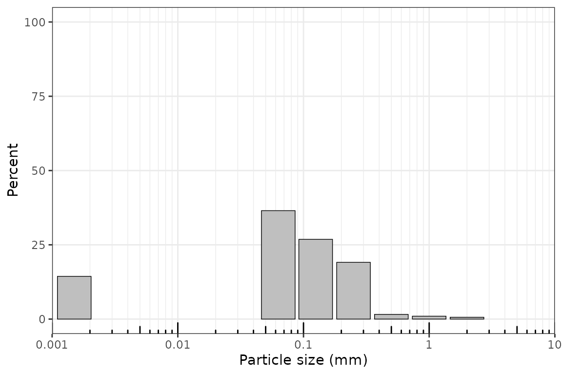
plot_distribution(gs_wide, sample = "S01", cumulative = TRUE)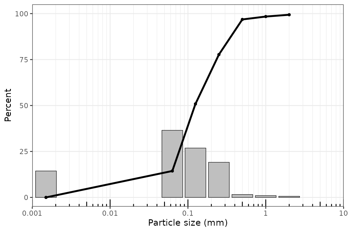
plot_distribution(gs_wide, x_scale = "phi", type = "line", sample = "S01")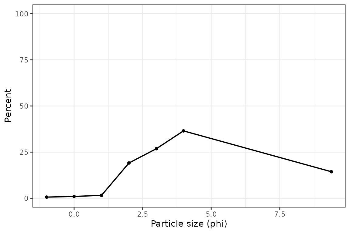
Cumulative Plots
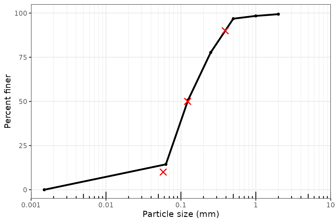
plot_cumulative() uses the same particle-size x-axis
conventions and can also add D-value markers.
suppressWarnings(plot_cumulative(
  gs_wide,
  sample_id = "S01",
  show_percentiles = c(10, 50, 90),
  extrapolate = "warn_linear"
))
Fraction Plots
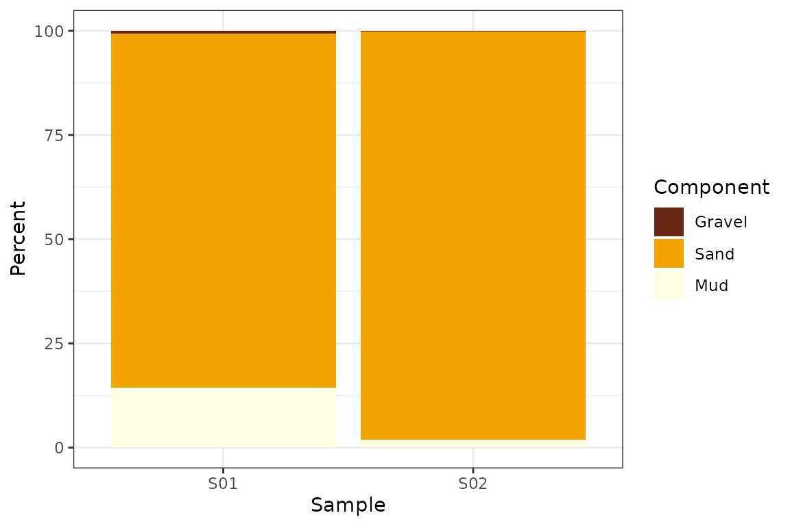
plot_fractions() draws size-class percentage bars. For
dry-sieve GRADISTAT-style examples, use non-overlapping
Gravel, Sand, and Mud fractions.
More detailed Wentworth-style classes are available with
scheme = "wentworth_detailed" when the input resolves those
boundaries.
plot_fractions(
  gs_wide,
  scheme = "gravel_sand_mud",
  sample_id = c("S01", "S02"),
  fill_palette = "YlOrBr"
)
Building a Combined Analysis Table
gs_parameters() collects common outputs into a single
table. More specialized helpers remain available when you need a
narrower result.
combined <- suppressWarnings(gs_parameters(
  gs,
  parameters = c("d_values", "d_spread", "folk_ward", "modes", "descriptors", "quality"),
  d_values = c(10, 50, 90),
  extrapolate = "warn_linear",
  moments_open_end = "extend_phi"
))

head(combined)
#> # A tibble: 6 × 82
#>   sample_id D10_um D50_um D90_um   D10   D25   D50   D75   D90 d_value_unit
#>   <chr>      <dbl>  <dbl>  <dbl> <dbl> <dbl> <dbl> <dbl> <dbl> <chr>
#> 1 S01         40.9   123.   390.  40.9  76.9  123.  233.  390. um
#> 2 S02         77.6   175.   412.  77.6 114.   175.  267.  412. um
#> 3 S03         69.5   151.   402.  69.5  91.3  151.  278.  402. um
#> 4 S04         60.2   125.   395.  60.2  81.2  125.  258.  395. um
#> 5 S05         62.2   123.   410.  62.2  80.1  123.  270.  410. um
#> 6 S06         76.1   216.   439.  76.1 104.   216.  346.  439. um
#> # ℹ 72 more variables: D90_D10_ratio <dbl>, D90_minus_D10 <dbl>,
#> #   D75_D25_ratio <dbl>, D75_minus_D25 <dbl>, D90_D10_log_ratio <dbl>,
#> #   D75_D25_log_ratio <dbl>, quartile_deviation_phi <dbl>,
#> #   any_extrapolated <lgl>, D5_um <dbl>, D16_um <dbl>, D25_um <dbl>,
#> #   D75_um <dbl>, D84_um <dbl>, D95_um <dbl>, D5_phi <dbl>, D16_phi <dbl>,
#> #   D25_phi <dbl>, D50_phi <dbl>, D75_phi <dbl>, D84_phi <dbl>, D95_phi <dbl>,
#> #   mean_fw_phi <dbl>, mean_fw_um <dbl>, sorting_fw_phi <dbl>, …
Notes on Open-Ended Tails and Extrapolation
Open-ended terminal classes are common in sediment data. grainsizeR does not silently turn them into closed intervals. Functions that need unresolved thresholds require an explicit extrapolation or open-end option, which makes the assumption visible in the analysis script.